Asset Management and Configurations Panel
This panel contains various sections that allow you to manage and configure different aspects of the asset, including segments, tags, metadata, label configurations, profiling, data freshness and other related settings.
Asset Details
In the Asset Details page, you can view the details of the current asset by clicking the  information icon.
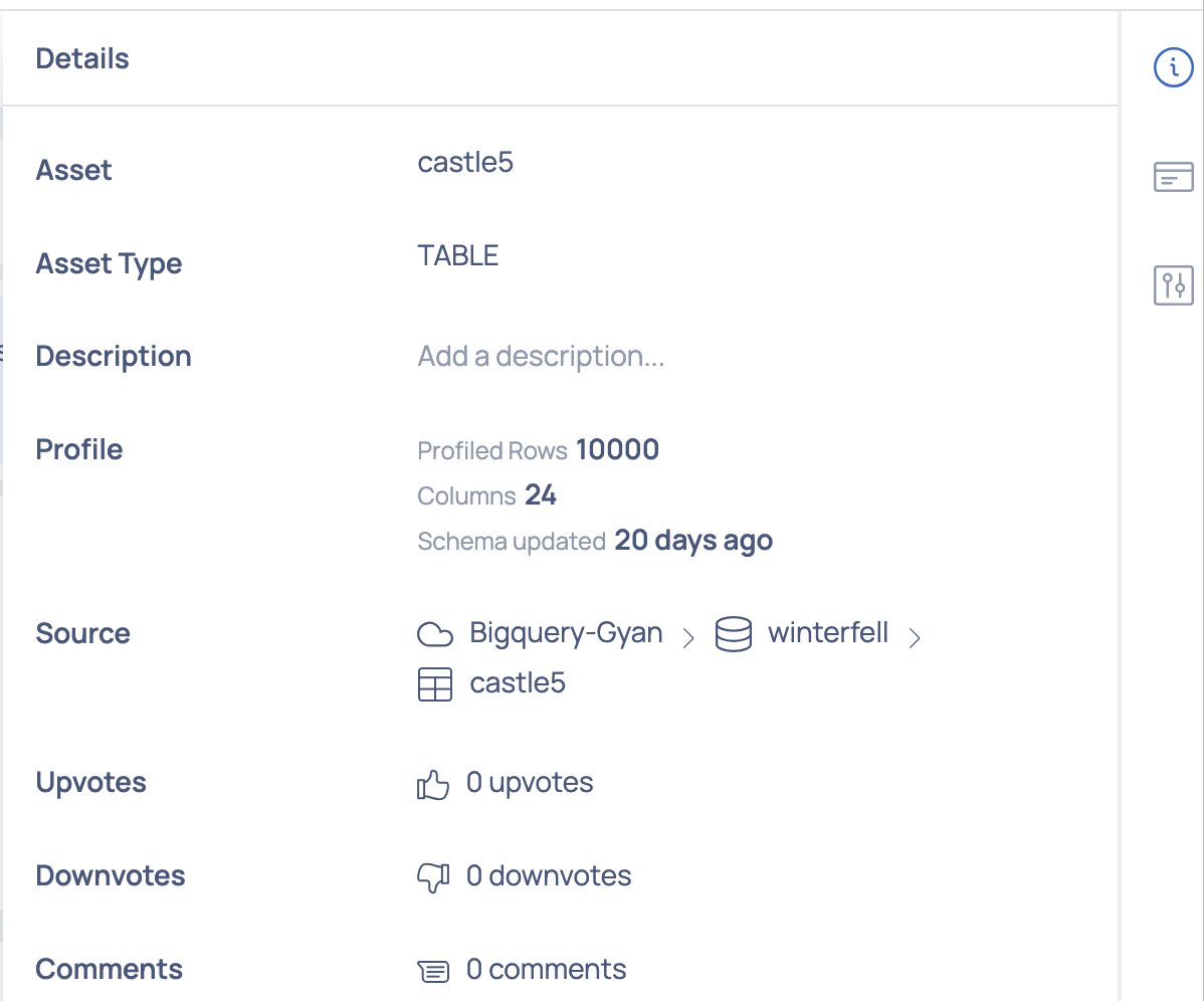
The following details of the asset can be viewed:
| Detail | Description |
|---|---|
| Asset | Displays the asset's name. |
| Asset Type | Displays the asset's classification, such as database, schema, table, or column. |
| Description | Offers a field to optionally provide an asset description. |
| Profile | Displays the detailed profiling data according to the asset type. For instance, for a table asset, the profiling information encompasses row count, column count, and days since schema update. |
| Source | Displays the asset's source path. |
| Upvotes | Displays the count of approvals received for the asset. |
| Downvotes | Displays the count of disapprovals received for the asset. |
| Comments | Displays the number of comments contributed to the asset. |
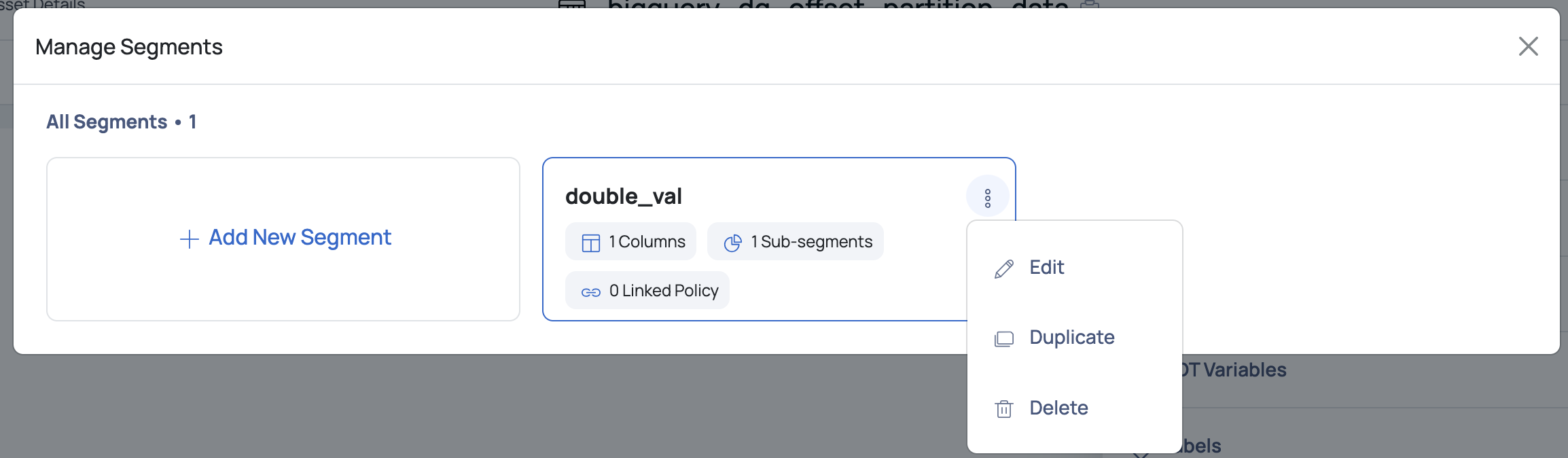
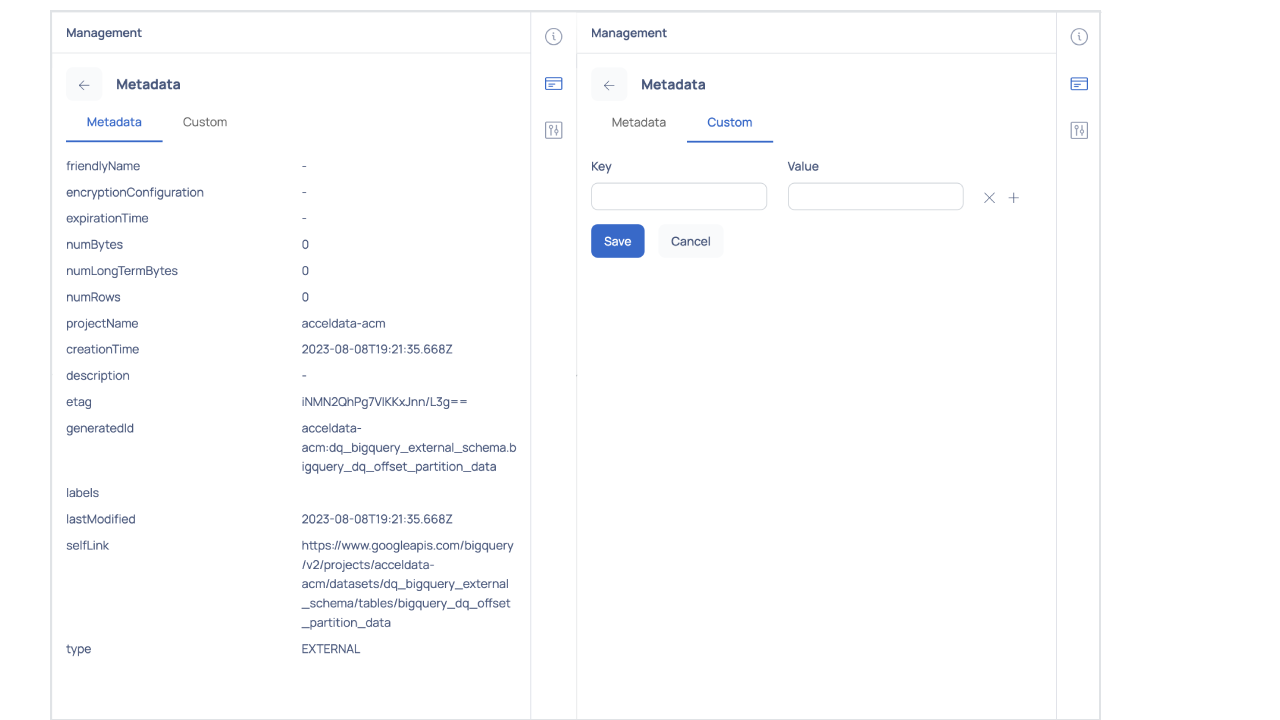
Management
Click to view the management modal window which allows you to perform the following actions based on the asset type:
Segment
Displays the existing segments created on the asset and also allows you to create new segments.
Tags
Displays the list of tags created on the asset. Click the Add tags button to add a new tag to the assets.
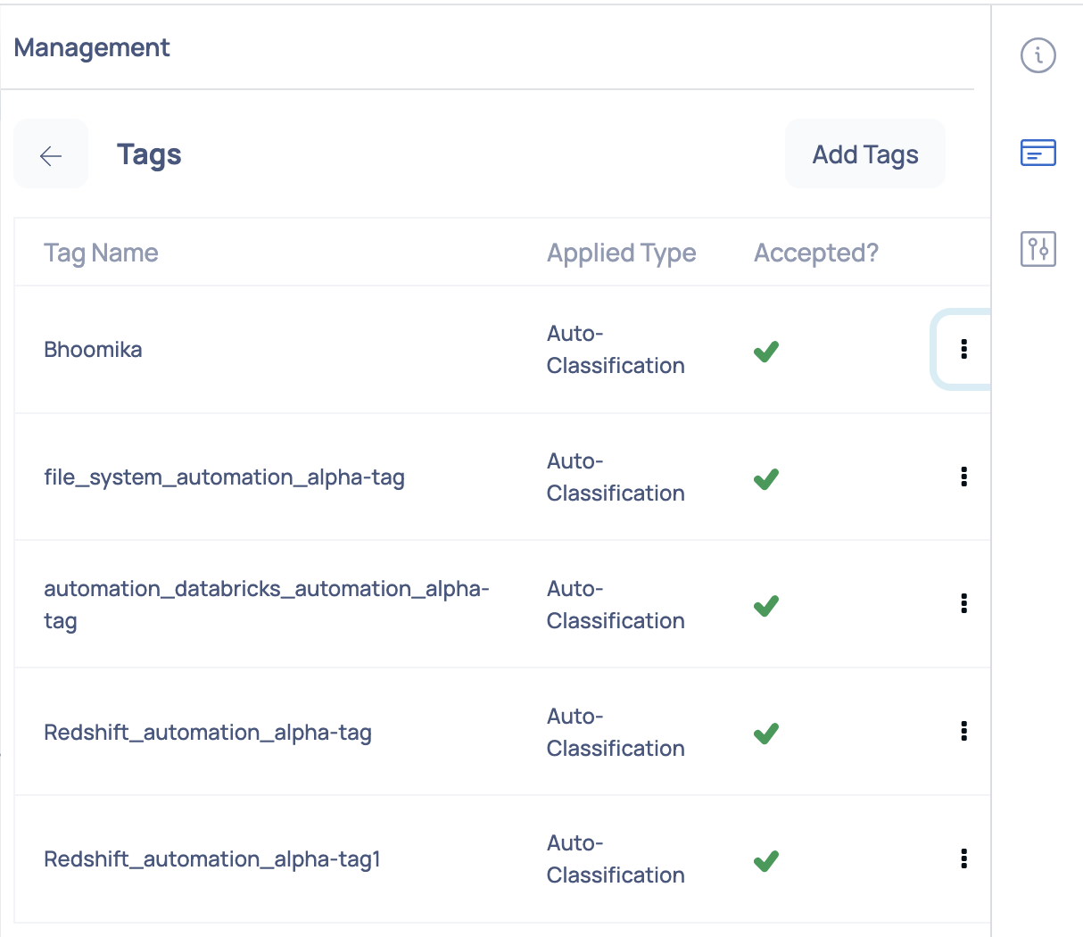
Tag Management
Metadata
Displays the metadata information about the asset. Click on the Custom tab to add custom metadata to the asset.
UDT Variables
Displays the (Link Removed) created on the asset.
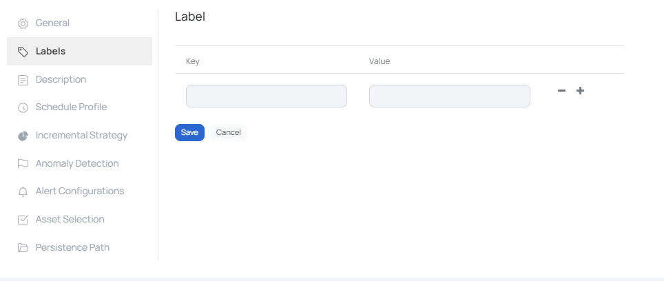
Labels
Labels are used to group assets. The Labels panel under the Settings tab, displays a table with the existing labels.
To add Labels, click the ADD button. Enter the Key and Value pair and click the Save button.
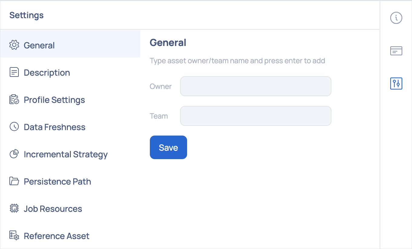
Settings
The user can add descriptions and labels to the asset, schedule profiling, configure an incremental strategy and add other configurations to an asset in the  Settings modal window.
Asset Details Settings Window
The Settings window displays the following configurations:
General
The

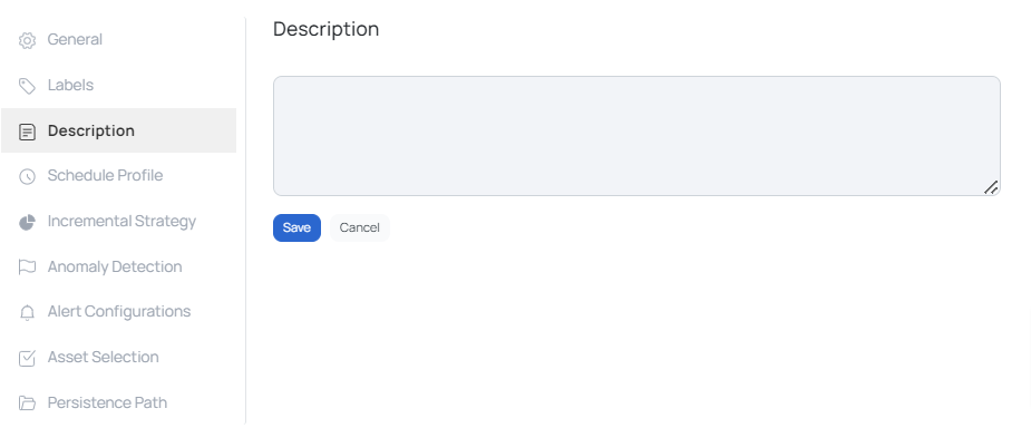
Description
The Description panel displays the description of the asset that was provided by the user while creating the asset. If a description does not exist for the asset, click the Add button to add one.
Enter the description and click the Save button.
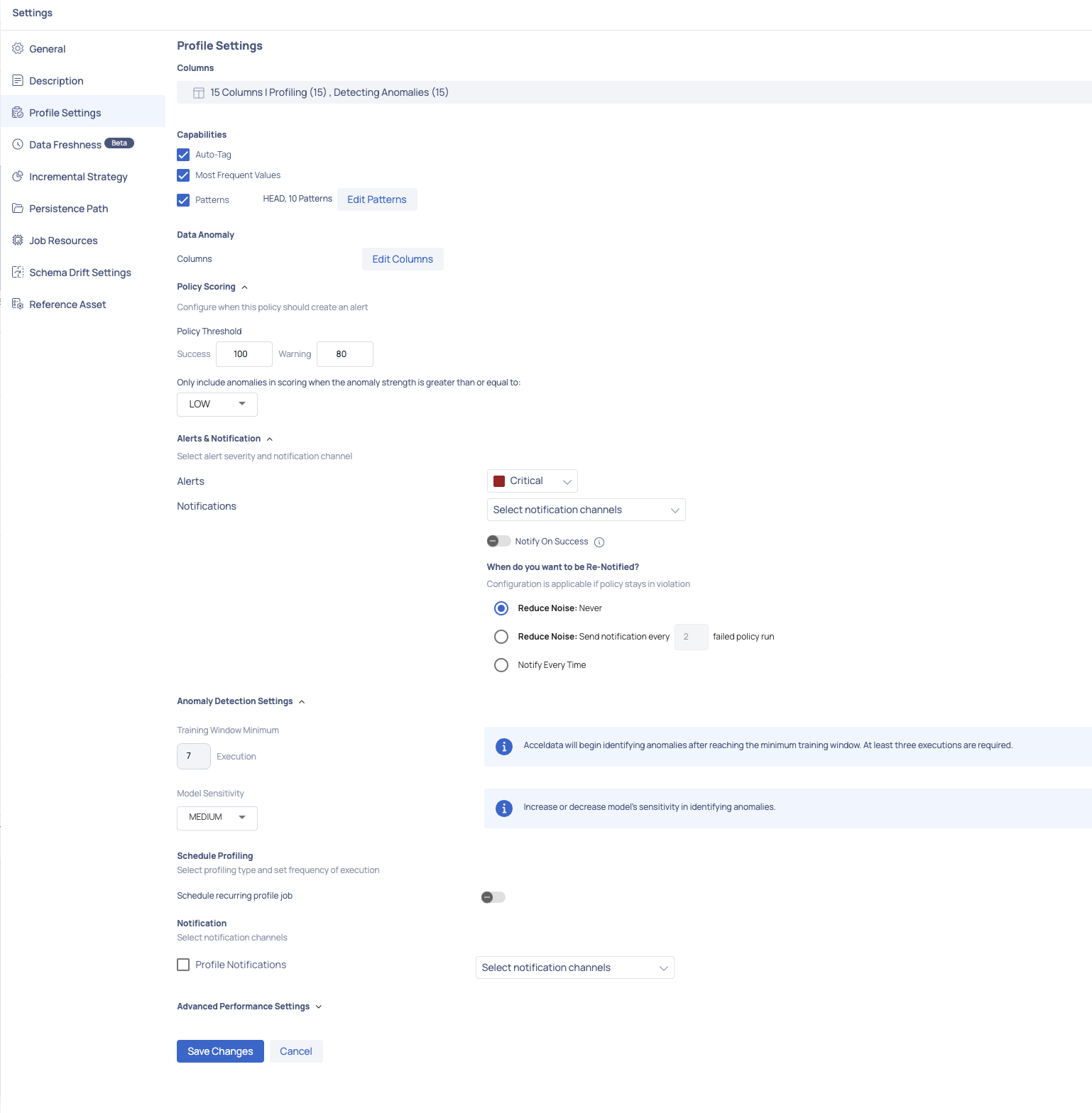
Profile Settings
One of the key features in the ADOC V3.4.0 release is the Profile Settings - Column selection tool in the data discovery module, which is specifically designed to optimize data profiling by allowing users to selectively target specific columns for profiling and anomaly detection.
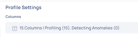
The Profile Settings interface displays the total number of columns available, as well as a breakdown of how many are set for profiling and anomaly detection.
Columns Selection Feature
Traditionally, profiling an asset in a data reliability project involved analyzing every column, which could be costly and often unnecessary.
Consider a scenario where a customer has an asset with a thousand columns. With the Profile Settings, they can choose to only profile the 600 relevant columns, effectively cutting down the cost and increasing the efficiency of their data profiling operations.
Now, with the feature, users can:
- Selectively Profile Columns: Choose only the relevant columns for profiling from potentially large datasets, avoiding unnecessary processing.
- Detect Anomalies Efficiently: Specify which columns to monitor for anomalies, streamlining the process and focusing on the most impactful data.
- Cost and Time Effective: Reduces the resources required for profiling by focusing only on selected columns.
Using the Columns Setting
- Navigate to Reliability > Data Discovery.
- Select an asset.
- Access Settings from the right-side menu.
- Enter Profile Settings.
- Here, users can click on the Columns option to select columns for profiling or anomaly detection.
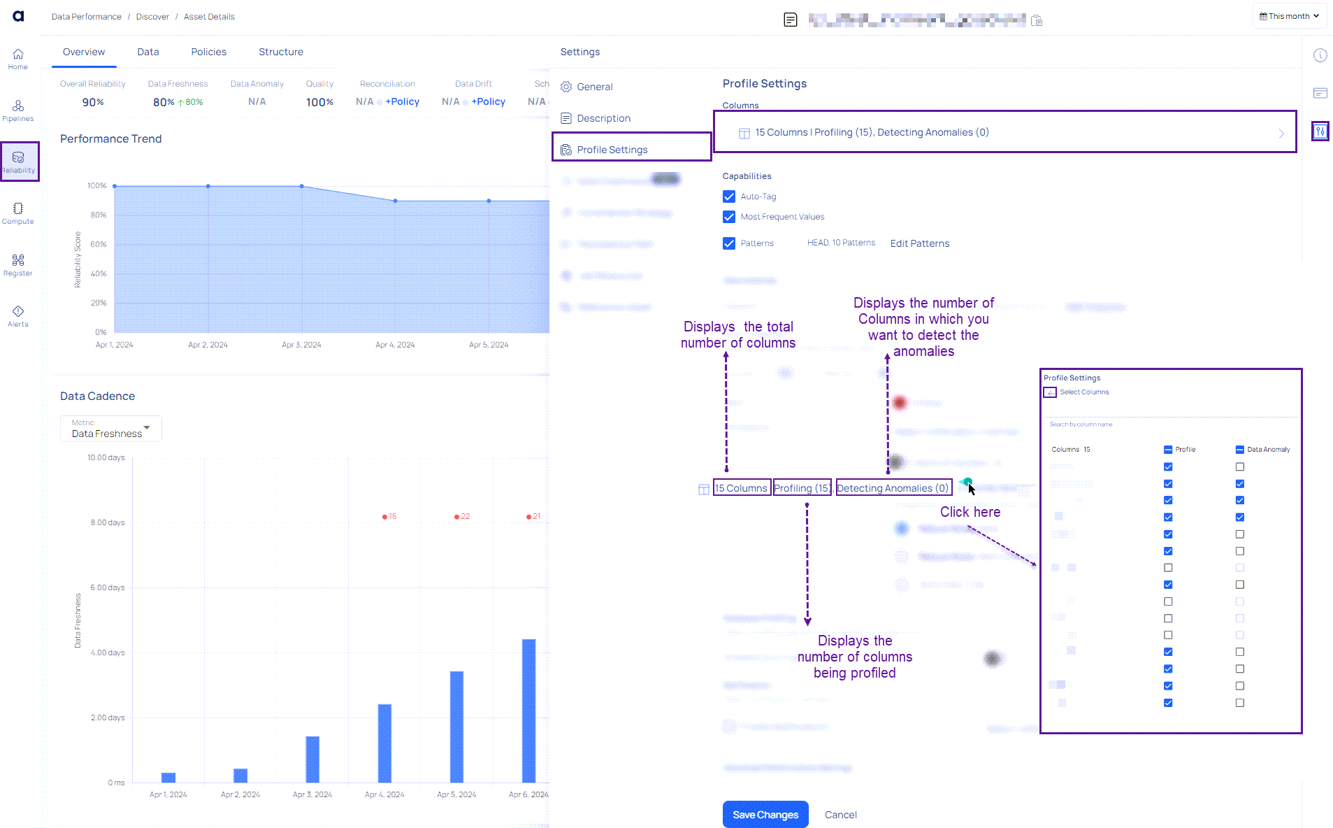
- Once selections are made, click the Back button to return to profile settings.
- Only columns with Profile enabled can have Data Anomaly selected; otherwise, the option remains inactive.
The Profile Settings window also allows you to configure the following capabilities for an asset:
- Auto-Tag
- Most Frequent Values
- Patterns
Data Anomaly
You have the option to activate data anomaly detection and choose the notification behavior.

Users can enable data anomaly detection in ADOC to boost data profiling capabilities. This feature detects hidden data irregularities, hence improving data quality and reliability. Turning on the toggle button
You can define the threshold for data anomaly policy by selecting the Policy Threshold option.
By clicking the Alerts button, you may specify which sort of abnormality should generate an alert.
Notifications allows you to choose which channels you want to be notified about.
The Columns section displays the various columns of the profile that are visible in a selected profile. You may select which columns will be checked for anomalies by clicking on the Edit Column button. Profiling is performed by default for all columns in the asset. You can, however, select the columns for anomaly detection based on your needs.
Enhanced data profiling capabilities from ADOC V2.12.1 onwards to enable the detection of anomalies in profile metrics for semi-structured data types. This update enables greater in-depth monitoring and analysis of your data assets.
Anomaly Detection Settings
Training Window Minimum: This is the minimum timeframe used to train anomaly detection for improved accuracy. A minimum training period of three days or more can be selected, during which any anomalies detected will not be considered for training.
Model Sensitivity: You can select the sensitivity level of the model—low, medium, or high. High sensitivity displays only high severity anomalies, medium sensitivity considers both medium and high severity anomalies, and low sensitivity shows all detected anomalies. The strength of each anomaly detected will be displayed based on the selected sensitivity level during execution.
Make sure to enable Data Anomaly for the columns to configure the Anomaly Detection Settings.
Schedule Profiling
You can schedule the profiling of an asset. To schedule profiling, perform the following steps:
- Enable the Schedule recurring profile job toggle button.
- Select one of the following profiling types from the Profiling Type drop-down list:
| Profiling Type | Description |
|---|---|
| Full | Profiles all the columns in the table. |
| Incremental | Incremental profile uses a monotonically increasing date column to determine the bounds for selecting data from the data source. |
When selecting Full Profile, you must schedule the profiling by choosing a time frequency—such as hour, day, week, or month—from the drop-down list and selecting the appropriate time zone.
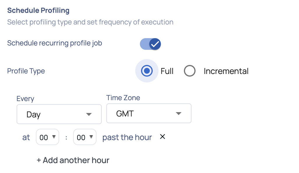
On selecting Incremental profiling, you must define an incremental strategy and then schedule the profiling by selecting the time from the drop-down list.
Notification
To receive profile notifications for an asset perform the following:
- Select the Profile Notifications checkbox.
- Click the Select notification channels drop-down and select all the channels that you would like to be notified on.
- Enable the Notify on Success toggle button to be notified if a profile on the asset was successful. By default you are notified if a profile on an asset fails.
- Click Save Changes to apply your profile configurations to the asset.
Handling Schema Changes in Data Profiling
ADOC's data profiling capabilities are designed to adapt dynamically to changes in your data schema. When new columns are added to an asset or existing columns are removed, ADOC's profiler can continue to function without the need for an immediate re-crawl of the asset. This ensures that schema changes will not disrupt your primary data flows, especially for data sources with challenging schema detection issues.
Profiling with Schema Changes
When profiling data with a schema update since the last crawl
For Missing Columns: If the profiler encounters a column present in the catalog but missing in the current data, it will skip profiling for the column without causing the entire process to fail. Results for those columns will not be generated.
For New Columns:
- Primitive Data Type: When a new column is of a primitive data type, the profiler will include it in the profiling results as expected.
- Complex Data Types: If the new column is of a complex data type (such as array, map, or structured data types) and Spark can natively detect these types, the profiler will attempt to generate semi-structured statistics.
Considerations for Semi Structure Data
For data sources, if a new complex column is introduced but not recrawled, Spark will receive those complex columns as strings (e.g., Snowflake data types Variant, Object, Array, etc.). Profile results will be presented as string statistics rather than semi-structured statistics. You will be able to obtain semi-structured statistics after recrawling and profiling.
User Action Required
While ADOC's profiler can handle schema modifications, to effectively utilize ADOC's data profiling features for semi-structured data, you should re-crawl the asset to update the catalog with the most recent schema.
This phase is critical for semi-structured data in order to obtain accurate and detailed profiling statistics.
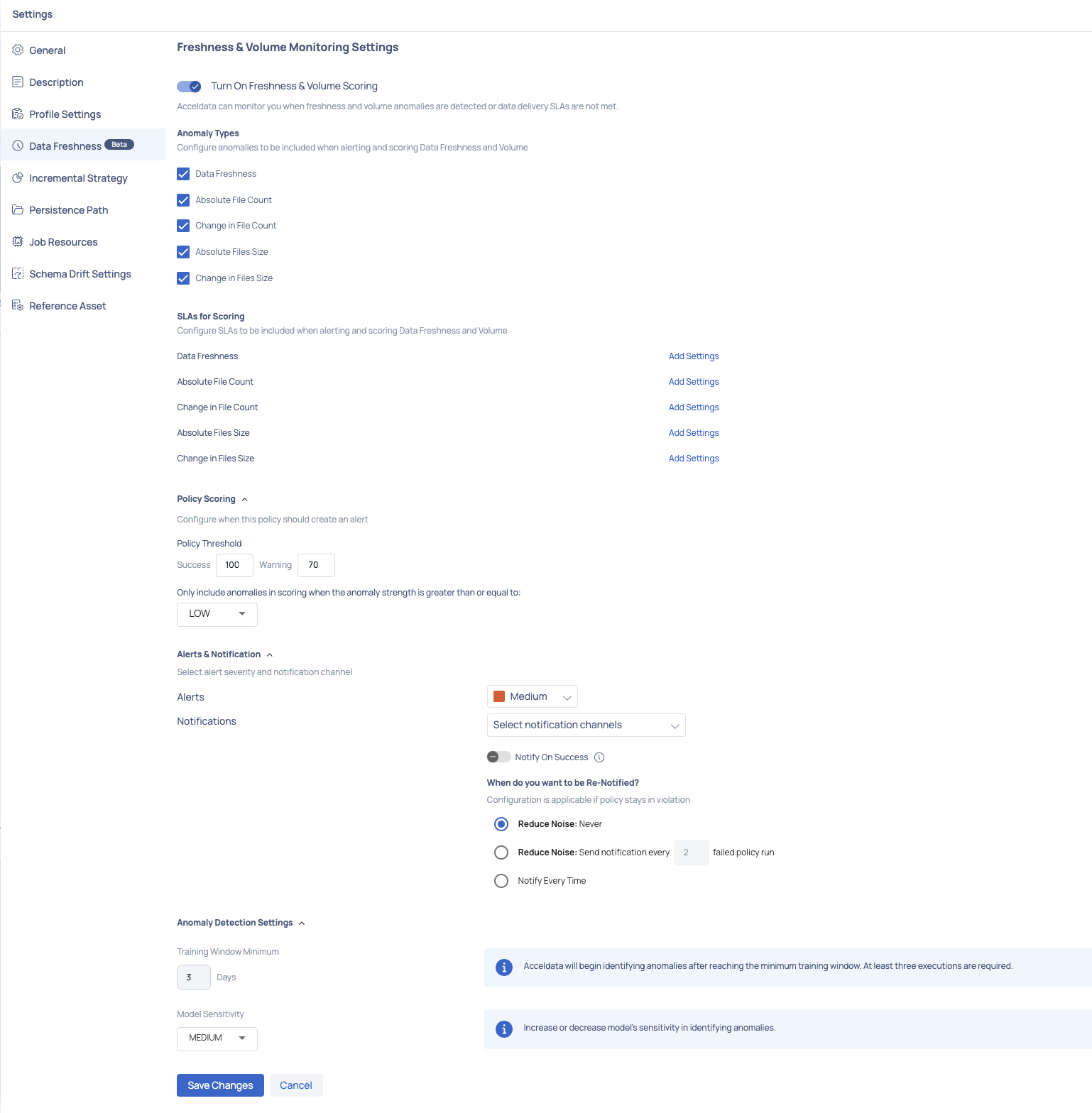
Data Freshness
The option for data freshness settings enables you to observe instances where anomalies in freshness and volume are identified, or when data delivery Service Level Agreements (SLAs) are not fulfilled.
Data Freshness is only calculated for the following asset types: Table and File
To turn on the freshness and volume monitoring settings, perform the following steps:
- Navigate to the asset details page of the selected asset.
- Click the asset Settings icon from the right.
- Click Data Freshness from the left menu bar. The Freshness & Volume Monitoring Settings is displayed.
- Enable the Turn On Freshness & Volume Scoring toggle button.
Anomaly Types
Select the following anomaly types to be included when alerting and scoring data freshness and volume:
- Data Freshness: Enable this checkbox to identify any anomalies in the updated data.
- Total Record Count: Enable this checkbox if you are monitoring a database asset to identify any anomalies in the total count of rows being processed.
- Change in Record Count: Enable this checkbox if you are monitoring a database asset to identify any anomalies in the count of rows as the database gets updated.
- Total File Count: Enable this checkbox if the asset is of file type to identify any anomalies in the total count of files being processed.
- Change in File Count: Enable this checkbox if the asset is of file type to identify any anomalies in the file count as newly added files are being processed.
- Total Data Volume: Enable this checkbox to identify any anomalies in the total volume of the data.
- Change in Data Volume: Enable this checkbox to identify any anomalies when there is change in data volume.
SLAs for Scoring
This section allows you to configure the following SLAs that need to be included when alerting and scoring data freshness and volume:
Data Freshness
Click the Edit Settings link to navigate to the Custom Threshold: Data Freshness pop-up. Enter the required values for the following parameters:
| Parameter | Values |
|---|---|
| Alert when update is not detected in the last | Enter an absolute number and click the Time Unit Selector drop-down to select either Days or Hours. |
Total Record Count, Change in Record Count, Total Data Volume, Change in Data Volume
For the remaining SLA configurations, click the Edit Settings link to navigate to the Custom Threshold pop-up. Enter the required values for the following parameters:
| Parameter | Values |
|---|---|
| Comparison | Select one of the following types of comparison for configuration of the SLA: User Defined or Relative |
| Alert when value | User Defined: For this type of comparison, click the dropdown menu and choose either the "Increases" or "Decreases" option, then enter the corresponding absolute value. Relative: If you prefer this comparison approach, click the dropdown menu and select either "Increases" or "Decreases," followed by inputting a percentage value. |
| Time Span | Relative: For this type of comparison, select either Hour or Day from the drop-down. |
| Compare Avg. over Last | Relative: Provide the value for the above time span type selected. |
Alerts and Notifications
- Enable the Alerts checkbox and choose the severity level for the alert.
- For receiving notifications, mark the Notifications checkbox and pick the notification channels through which you wish to receive updates. Enable the Notify on Success toggle to receive notifications when the policy execution is successful.
- Define the success threshold values for both success and warning statuses.
Anomaly Detection Settings
Training Window Minimum: This is the minimum timeframe used to train anomaly detection for improved accuracy. A minimum training period of three days or more can be selected, during which any anomalies detected will not be considered for training.
Model Sensitivity: You can select the sensitivity level of the model—low, medium, or high. High sensitivity displays only high severity anomalies, medium sensitivity considers both medium and high severity anomalies, and low sensitivity shows all detected anomalies. The strength of each anomaly detected will be displayed based on the selected sensitivity level during execution.
Make sure to enable the Turn On Freshness & Volume Scoring toggle to configure the Anomaly Detection Settings.
Complete the process by clicking the Save Changes button to save the modifications made above.
After enabling data freshness and saving your changes, a data freshness policy is established for the asset. This policy will execute every hour to ensure the up-to-date status of the data.
Viewing Results of Data Freshness Policy Executions
To view the execution results of a data freshness policy that is enabled for an asset, perform the following:
- Navigate to the left menu and click Reliability > Policies to proceed to the Policies page.
- Search for the asset's name where the policy is enabled, or utilize the Policy Type dropdown to select Data Freshness, revealing all the assets under this policy.
- Click on the asset's name to be directed to the Policy Executions page, where you can explore execution details.
The left-hand side presents a timeline of asset policy executions, along with the data freshness score. To access execution specifics, click on any execution, and details will appear on the right. Three panels are available:
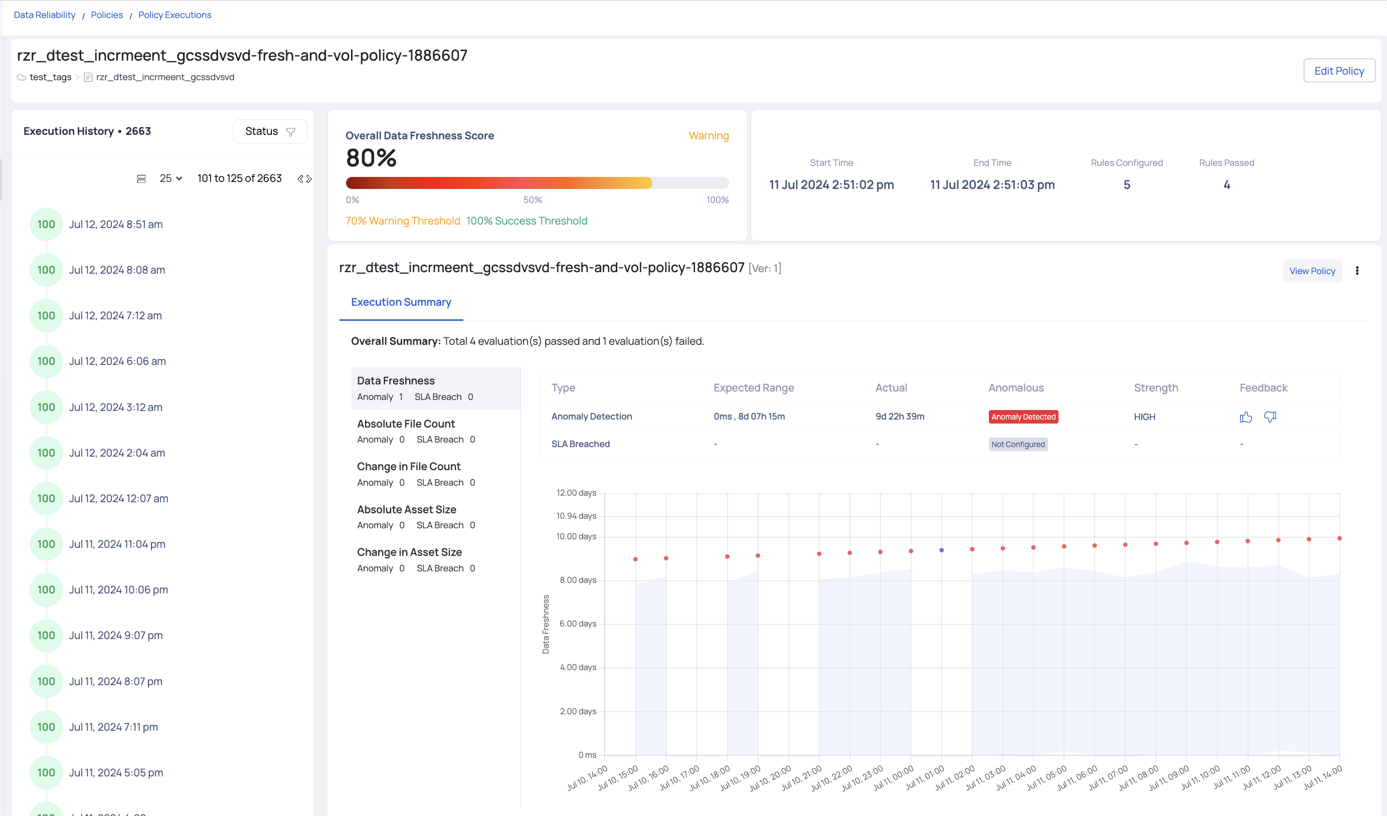
- Overall Data Freshness Score: This panel displays the execution status (errored, warning, or successful) and the score as a percentage from 0 to 100.
- Details: The second panel provides Start Time, End Time, Rules Configured, Rules Passed, and Execution Type.
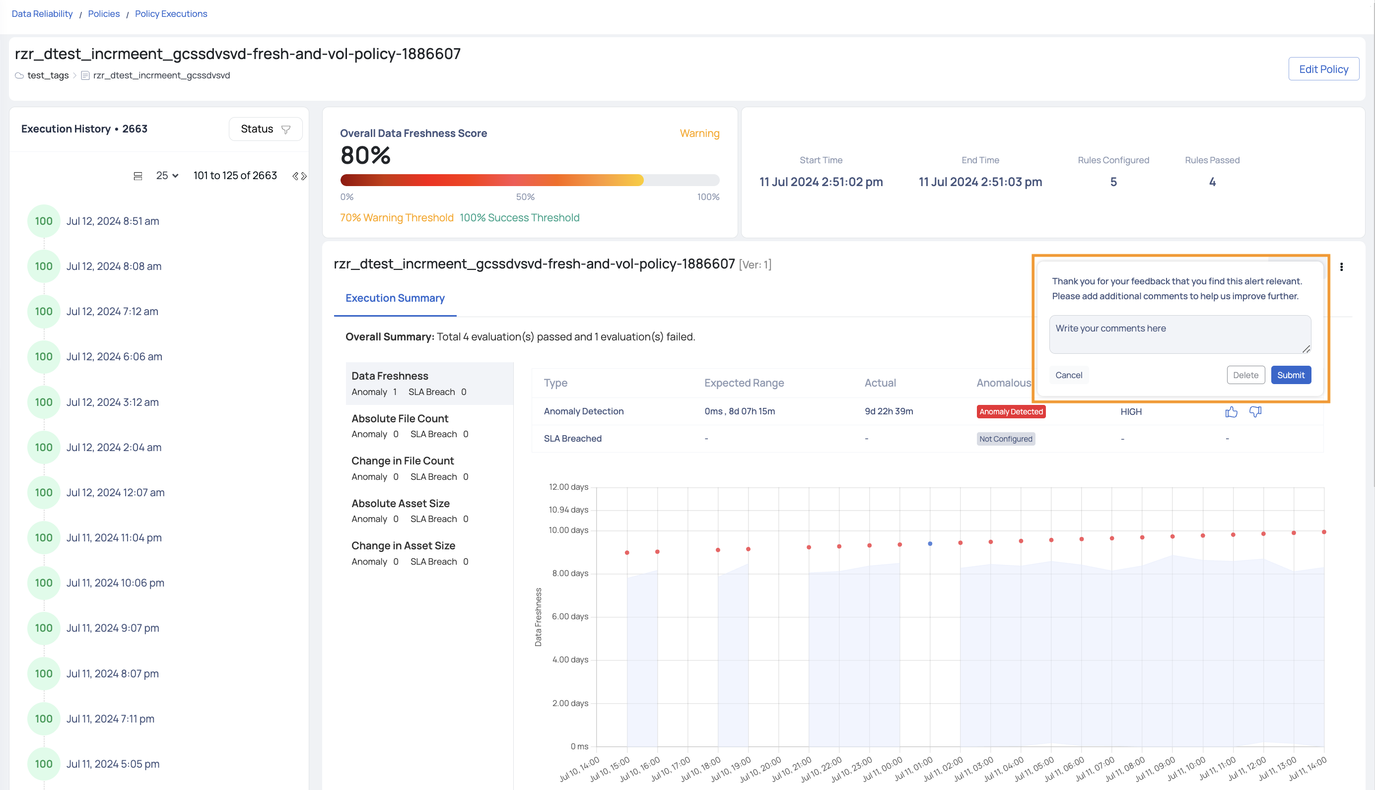
- Execution Summary: Here, you'll find a comprehensive view of configured rules, along with detected anomalies and SLA breaches for each rule. An accompanying table offers Expected Range and Actual values details. The strength of the anomaly will also be highlighted accordingly. Additionally, users can provide feedback on each detected anomaly, indicating whether they agree with the detection or believe it was inaccurate. This feedback helps improve the accuracy of future anomaly detections and ensures the system continuously learns and adapts to user needs.
Viewing Detected Anomalies
Upon executing the data freshness policy, if anomalies are identified, they can be reviewed on the Asset Details page using the following steps:
- Navigate to the Asset Details page of the asset.
- Click Data > Cadence.
Anomaly detection will be enabled three days after adding the data source. This waiting period allows us to accumulate sufficient data before classifying any metrics as anomalies.
The Freshness Trend chart illustrates data gaps within the chosen timeframe. You can select a y-axis value like absolute row count, change in row count, absolute asset size, or change in asset size. A graph is presented reflecting data for the chosen period. For instance, if you opt for change in row count as the y-axis and the chosen timeframe is the current month, the graph will display row count changes for each day of the month. Detected anomalies are marked with orange dots alongside a corresponding number indicating the count of anomalies. Clicking on an orange dot allows for further exploration, revealing the exact time of anomaly occurrence, along with upper and lower bounds, and the specific y-axis value.
Incremental Strategy
The user can profile an asset incrementally, that is, first profile a number of rows and then profile successive rows. For incremental profiling, you must define an incremental strategy. Acceldata Data Observability Cloud (ADOC) supports following types of incremental strategies, namely:
- Auto Increment Id based
- Partition based
- Incremental date based
- Incremental file based
- Time stamp based
To define an incremental strategy at the asset level, click the Settings tab of the asset, then select Incremental Strategy. The following section explains the three types of incremental strategies, along with the required inputs:
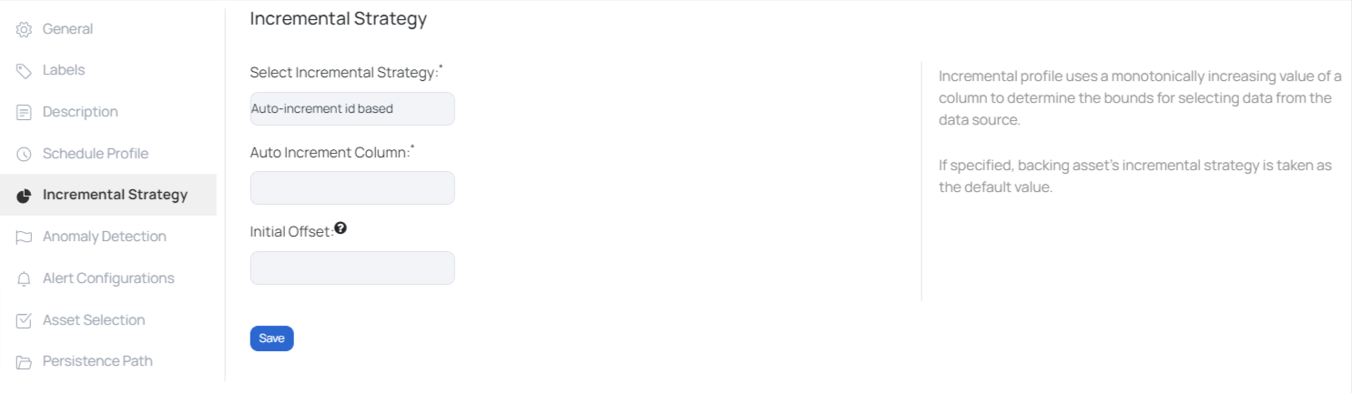
Auto Increment Id Based
Incremental profile uses a monotonically increasing value of a column to determine the bounds for selecting data from the data source.
For example, every time a new row or rows of data are added to the database, they are allotted with an auto-incrementing numeric value. For instance, on adding 1000 rows of data to the database, each row is given an id starting from 1 to 1000. When the data source is profiled, the first 1000 rows are taken into consideration. Let's say you added another thousand rows of data to the database. An auto increment id based strategy is used to provide values from the last incremented value of the preceding set of rows, i.e., 1001 to 2000. On profiling, only the new set of rows are profiled.
The following table describes the required inputs:
| Input Required | Description |
|---|---|
| Auto Increment Column | Select the auto increment column. |
| Initial Offset | If a value is specified, then the starting marker for the first incremental profile will be set to this value. If left blank, then the first incremental profile will start from the beginning. |
Partition Based
Incremental profile uses a date based partition column to determine the bounds for selecting data from the data source. The required inputs varies depending on the type of Sub Strategy selected. Currently there are two types of sub strategies, namely:
- default
- day-month-year
Default - Sub Strategy
Incremental profile uses a date based partition column to determine the bounds for selecting data from the data source. Only useful if the data source supports partition. The required inputs are as follows:
- Partition Column: Select the partition column
- Day Format: Provide a date format to save the date timestamp. For example, YYYY-MM-DD
- Frequency: The profiling frequency can be set to hourly, daily, weekly, monthly, quarterly and yearly.
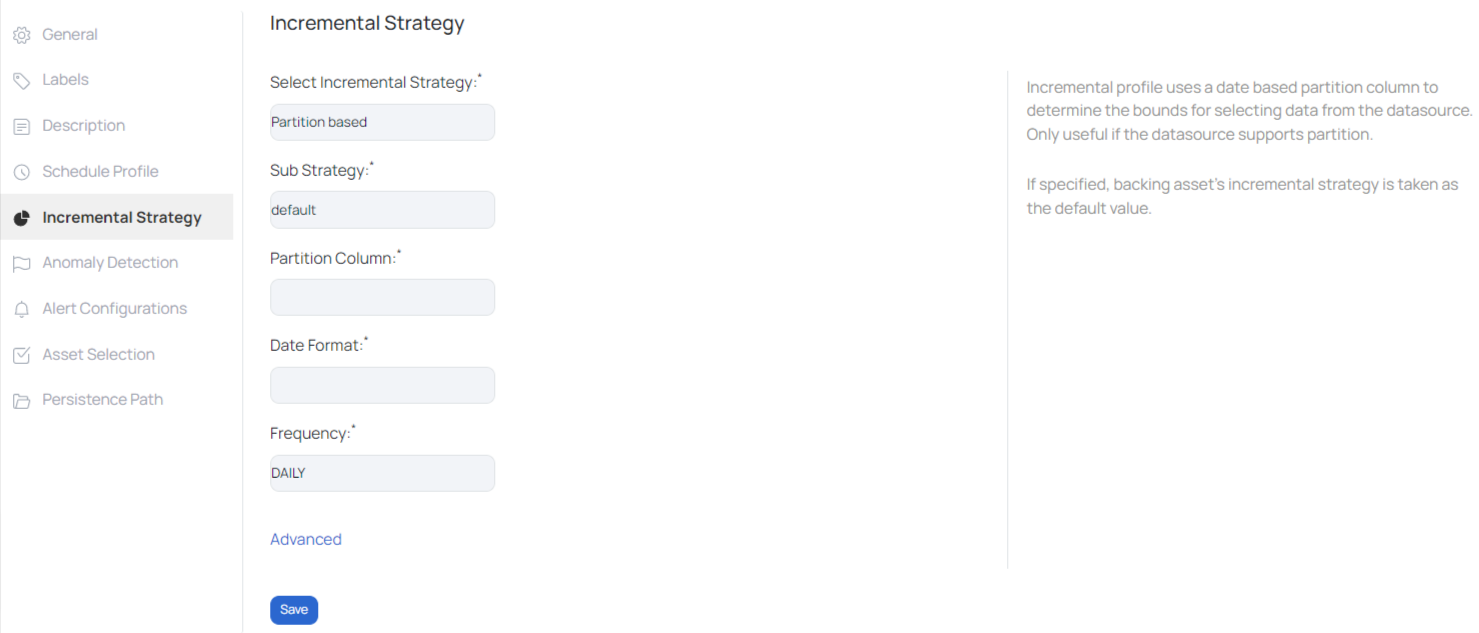
For more options, click on Advanced. Enter the following data under the advanced fields:
- Time Zone: Select a time zone from the drop-down list.
- Offset: If the selected time zone is offset by a few hours or minutes, then enter the number of hours or minutes in the field provided.
- Data Prefix: If the selected partition column has some prefix attached to its values, then specify the prefix data.
- Data Suffix: If the selected partition column has some suffix attached to its values, then specify the suffix data.
On checking Round End Date, the last executed date value is rounded up by the frequency that is selected from the Frequency drop-down list for the next execution of the policy. For instance, at 12:20, the last data row was executed, and you checked Round End Date and selected Hourly frequency. Therefore, the next time the policy is executed, it will only be executed on the data created at 13:20 and so on.
Click the Save button.
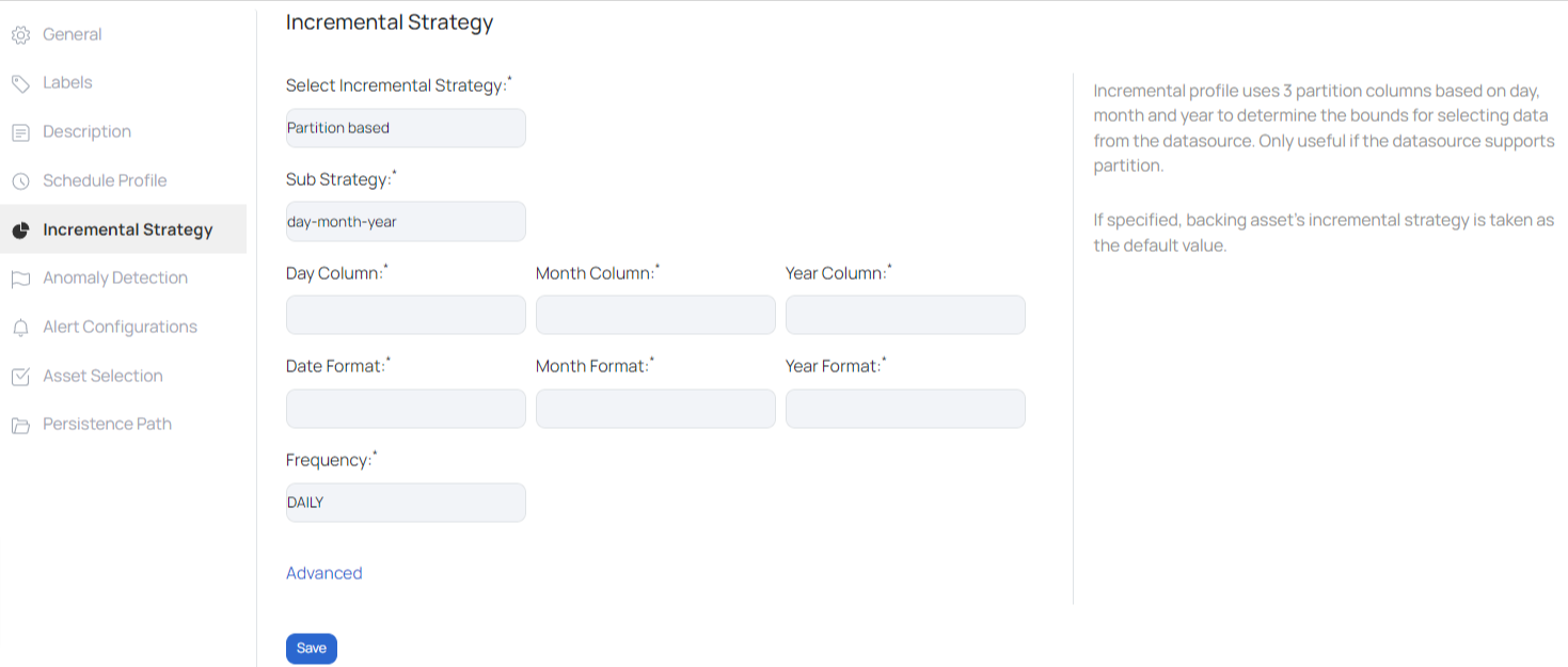
Day-month-year - Sub Strategy
Incremental profile uses three partition columns based on day, month and year to determine the bounds for selecting data from the data source. Only useful if the data source supports partition.
The required inputs are as follows:
- Day Column: Date based partition column
- Month Column: Month based partition column
- Year Column: Year based partition column
- Day Format: Provide a date format. For example, DD
- Month Format: Provide a month format. For example, MM
- Year Format: Provide a year format. For example, YY
- Frequency: The profiling frequency can be set to hourly, daily, weekly, monthly, quarterly and yearly.
For more options, click on Advanced. Enter the following data under the advanced field:
- Time Zone: Select a time zone from the drop-down list.
- Minute Offset: If the selected time zone is offset by a few hours or minutes, then enter the number of minutes in the field provided.
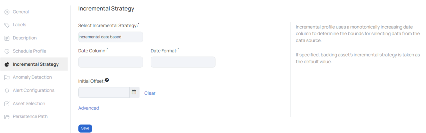
Incremental Data Based
Incremental profile uses a monotonically increasing date column to determine the bounds for selecting data from the data source. The following table describes the required inputs:
| Input Required | Description |
|---|---|
| Date Column | Select the column name that is used to save dates and timestamps. |
| Date Format | Provide a date format to save the date timestamp. For example, YYYY-MM-DD |
| Initial Offset | If a date is specified, then the starting marker for the first incremental profile will begin from the specified date. If left blank, then the first incremental profile will start from the beginning. |
For more options, click on Advanced. Enter the following data under the advanced field:
- Time Zone: Select a time zone from the drop-down list.
- Minute Offset: If the selected time zone is offset by a few hours or minutes, then enter the number of minutes in the field provided.
On checking Round End Date, the last executed date value is rounded up by the frequency that is selected from the Frequency drop-down list for the next execution of the policy. For instance, at 12:20, the last data row was executed, and you checked Round End Date and selected Hourly frequency. Therefore, the next time the policy is executed, it will only be executed on the data created at 13:20 and so on.
Click the Save button.
Incremental File Based
When enabling the Monitoring File Channel Type for an asset in S3, GCS, or ADLS data source during configuration, the data plane's monitoring service actively searches for file events such as file additions, deletions, or renames on that specific data source. Once a file event is captured, it is forwarded to the catalog server, which then stores the event details.
To enable a file-based incremental strategy for an asset, go to the asset's details page, click on Settings from the right-hand side, and click Incremental Strategy from the left menu.
Incremental profile uses a monotonically increasing date column to determine the bounds for selecting data from the data source. The following table describes the required inputs:
| Input Required | Description |
|---|---|
| Initial Offset | If specified, the starting marker for the first incremental profile will be set to this value; if left blank, the first incremental profile will start from the beginning. |
| Time Zone | Select the desired time zone for configuring the initial offset. |
When the Round End Date checkbox is selected, the number of the most recent date the policy was run is rounded up by the frequency selected from the Frequency drop-down list for the next time the policy is performed. If you checked Round End Date and picked Hourly regularity, for example, the last row of data was processed at 12:20. As a result, when the policy is executed again, it will only run on the data created at 13:20, and so on.
Click the Save button.
Time Stamp Based
The Time Stamp Based Incremental Strategy allows users to incrementally profile an object using time stamps. This method profiles data in a chronological order, making it excellent for datasets with time-related data points. This technique establishes the bounds for data selection by employing a time-stamp column, guaranteeing that only fresh or altered data points (after the previous time stamp) are profiled throughout successive runs.
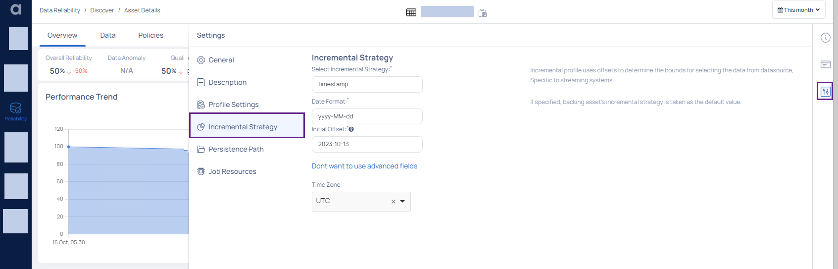
| Input Required | Description |
|---|---|
| Select Incremental Strategy | Choose the Time Stamp Based option from the dropdown to set your incremental strategy to Time stamp. |
| Date Format | Define the format in which the time stamp data is saved, e.g., YYYY-MM-DD HH:MM:SS. |
| Initial Offset | If specified, the starting marker for the first incremental profile will begin from this value. If left blank, the profiling starts from the beginning. |
| Time Zones | Choose the appropriate time zone based on the origin of the data or the intended audience for the profiling findings. This ensures that timestamp-based data profiling is correct. |
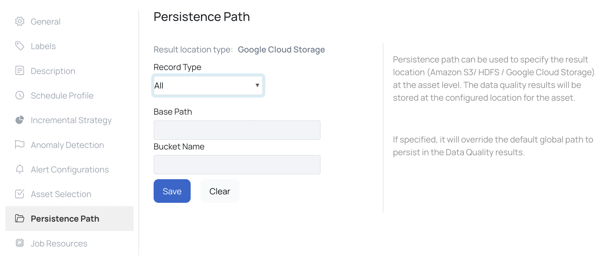
Persistence Path
Whenever you execute a data quality policy or a reconciliation policy, data violations are generated if the policy fails. Data Violations are rows of data that attributed to the failure of the policy. The user can choose to store this data violations in the desired location.
To configure the result location at the asset level, click the Settings tab of the asset, and select Persistence Path. Specify the Path and click the Save button.
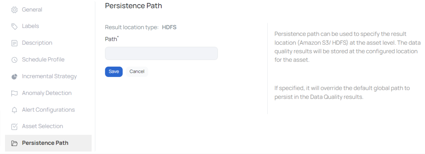
The result location type can either be HDFS, Google Cloud Support (GCP) or Amazon S3. This is configured in the analysis service. In case of Amazon S3, you must specify the following parameters:
- Bucket Name: Name of the S3 bucket
- Region: Name of the region
- Path: Path of the result location
Job Resources
This setting allows you to assign resources for Spark job executions. You can set resources like executors and CPU cores on this page.
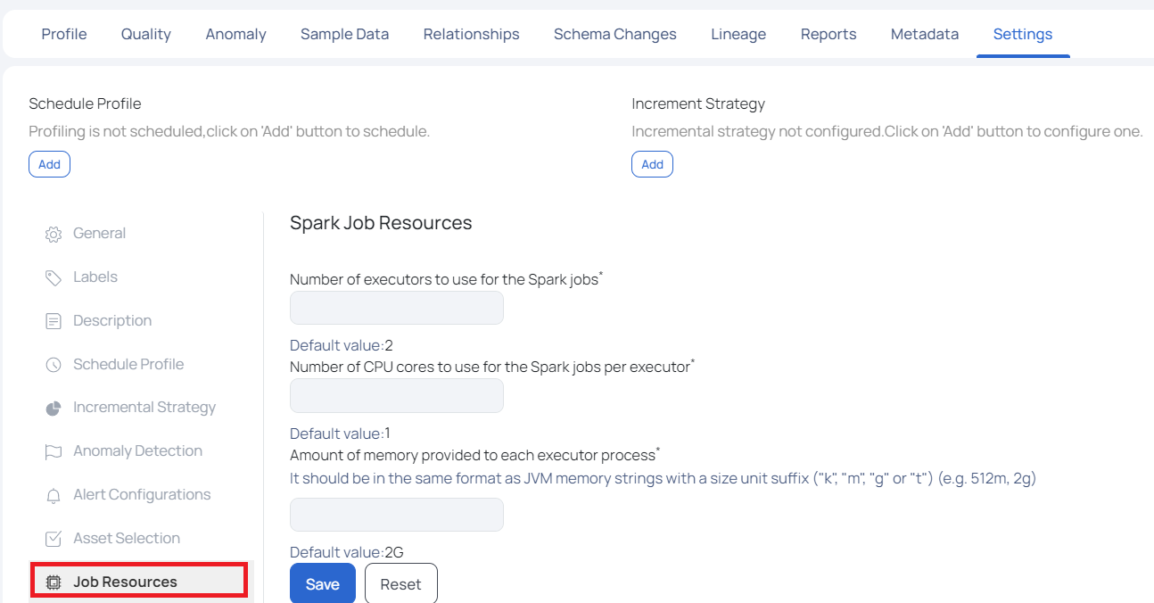
This page has the following settings.
- Number of Executors to Use for the Spark jobs: In this field, you must set the number of executors to be assigned for Spark jobs execution. By default, two executors are assigned.
- Number of CPU cores to use for the Spark jobs per executor: In this field, you must set the number of CPU cores to be assigned for Spark jobs execution. By default, one CPU core is assigned.
- Amount of memory provided to each executor process: In this field, you must set the amount of memory to be assigned to each executor process. The memory allocation must be in JVM memory strings format. By default, 2 GB memory is allocated.
Click Save once you have configured all the settings.
Schema Drift Settings
The Schema Drift Settings page in ADOC enables users to track and manage changes to their data schema. This involves recording column additions, removals, and revisions. The settings can be configured to notify users via various notification channels dependent on the severity of the identified changes.
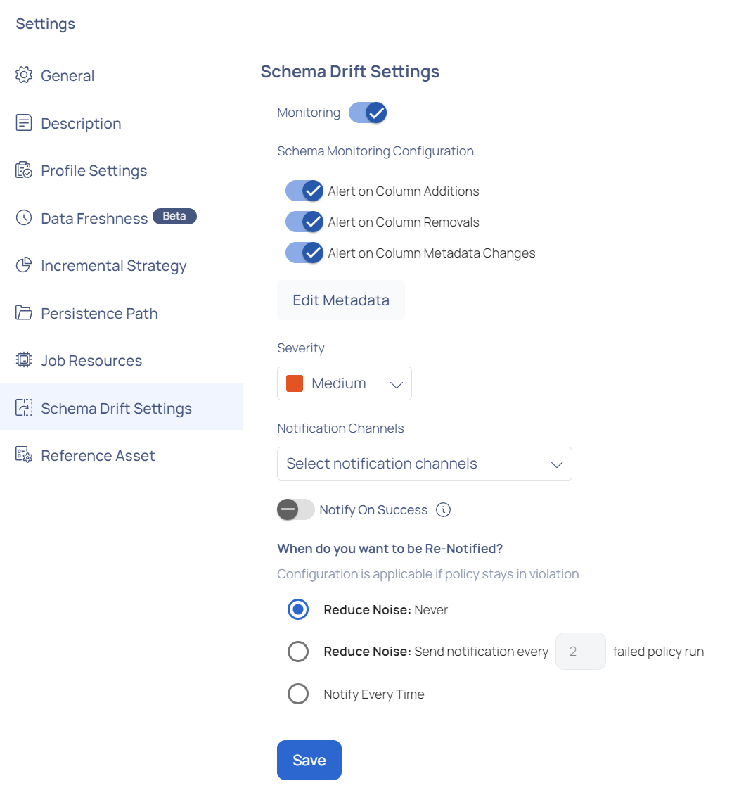
Monitoring: Toggle the Monitoring switch to enable or disable schema monitoring.
Schema Monitoring Configurations:
- Alert on Column Additions: Enable this to receive alerts when new columns are added to the schema.
- Alert on Column Removals: Enable this to receive alerts when columns are removed from the schema.
- Alert on Column Metadata Changes: Enable this to receive alerts for any changes in the metadata of existing columns.
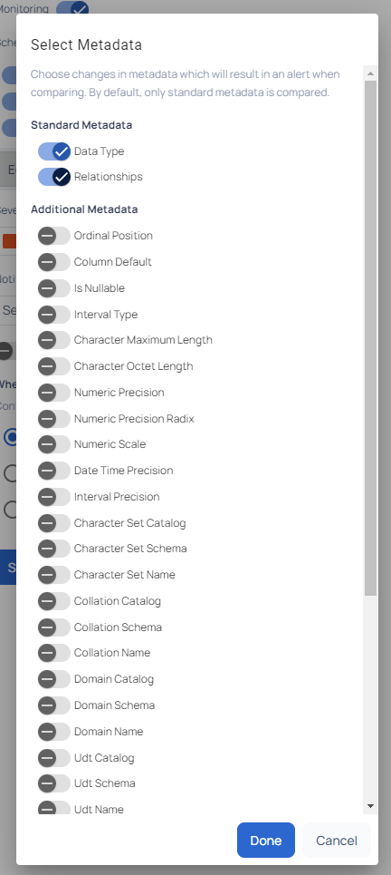
- Edit Metadata: Click this button to modify metadata settings for columns.
Click Edit Metadata to configure the specific metadata settings for each column.
This opens a Select Metadata tab where users can choose the types of metadata to monitor. By default, standard metadata such as Data Type and Relationships are selected. Users can also choose additional metadata from options like Ordinal Position, Column Default, Is Nullable, Character Set Name, Numeric Precision, and more.
Severity: Set the severity level of the alerts. Options typically include levels like Low, Medium, and High.
Notification Channels: Select the channels through which you wish to receive notifications (e.g., Email, Slack).
Notify On Success: Toggle this option to receive notifications even when the policy execution is successful.
Re-Notification Settings:
- Reduce Noise: Never: Select this to never send re-notifications.*
- Reduce Noise: Send notification every X failed policy run: Specify the number of failed policy runs before sending a re-notification.
- Notify Every Time: Select this to send a notification for every instance of policy violation.
- Regularly review and adjust the Severity level and Notification Channels to ensure timely and relevant alerts.
- Use the Reduce Noise settings to avoid alert fatigue by controlling the frequency of notifications.
- Ensure that the Notify On Success option is used judiciously to balance between getting comprehensive updates and avoiding unnecessary alerts.
Reference Asset
You can use this setting to mark the asset as a Reference asset. Reference assets can be used for Lookup in a Lookup rule in Data Quality policies. To learn more about this setting, see Lookup Data Quality Policy.